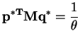
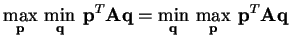
In other words,

is the amount of payoff that the row player is guaranteed to win on the average, assuming that he plays rationally.
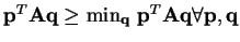
Lemma: For any matrix A,


 .
Proof
.
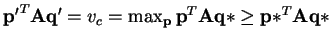
Proof :
We observe that
. Taking the maximum over all

on both sides,
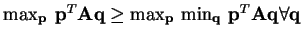
. The RHS is
, thus the previous equation can be re-written as
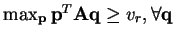
. Therefore
. This proves

.

:

is a Nash Equilibrium iff
.
Proof : (

) As
is a Nash Equilibrium of A,
. Also,
and
. Hence,
. Combining these two we get,

. But from previous lemma

. This proves

.
(

) Choose

s.t.,
. Now choose

s.t.
. Since

is the minimum over all
and

strategy

s.t.
.
Thus
.
Since

is the minimum over all
,
.
Thus

is also minimum over all
for the same

.
. Thus
is a Nash Equilibrium.
![$ \mathbf{ [Von Neumanns' Minimax Theorem]}$](img117.png)
For any two person zero-sum game specified by matrix

, optimal mixed strategies exist for both players. Moreover
the row and column values are equal. In other words,
 |
(1) |
or

.
Also if

and

denote the optimal strategies for the row and the column player respectively, then
-
- (,) is a Nash Equilibrium for this two player game.
The optimal strategy for row player will yield the same payoff as the optimal strategy for Column player! If either the row or the column player plays her optimal strategy, the opponent cannot improve the expected payoff. Thus once a player has
publicly committed to play the optimal strategy, it is possible for the other player to play the game with a pure strategy and still receive the optimal expected payoff.
This proof requires the duality theorem, a well known result in linear programming.
A linear programming problem can be defined in terms of constraints

and

, and a cost vector

. The goal is to minimize the cost

subject to the constraints and given a cost vector. This is called the
primal problem.
Associated with every primal problem is a
dual problem stated as follows.
The constraints now become

and

, the new cost vector is

and the goal is to maximize

.
![$ \mathbf{ [Duality Theorem]}$](img132.png)
If either problem (primal or dual) has a best vector (called

or

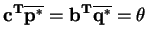
), then so does the other. The minimum

equals the maximum

 |
(2) |
In terms of

(the row player) and

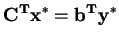
(column player), we want to minimize (primal)

(called

) subject to the constraints

and

. We also want to maximize (dual)

(called

) subject to the constraints

and

, where

and
are unit vectors. In light of this formulation and the duality theorem, we can state
 |
(3) |
Therefore, our probability distributions that correspond to our optimal vectors

and

are obtained by setting

and

.
[Proof of Von Neumanns' Minimax Theorem]
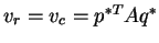
Since

,
. And since

, this implies that
. This gives a lower bound on how much
is winning (

). Similarly,
implies that
and that
is an upper bound on
's loss.
Therefore,