Hidden Line Removal
Skip this section
After seeing your reports for assignment (I), it seems that the major problem that has the majority of you grumbling is the Forward Problem. Specifically the Hidden-Line stuff. Majority of you have invested a good amount of creativity in coming up with several solutions. However it turns out that the correctness of quite a few of them are subject to closer perusal. This page is a chronicle of the discussion which we (myself and Avinash) had tonight (10th September) . What we present here is a sketch of an algorithm which to our sleep
laden minds appears to be correct. However we warn you that its correctness is to be established. Also counter examples are welcome and you can post them in the discussion list. Also Avinash feels that he has seen/read something like this somewhere, so any resemblance to any algorithm living or dead is purely co-incidental. Also this algorithm is inspired by an algorithm presented by someone in your class. We felt that it has some problems and this is the result of our effort to improve upon it.
The Problem
Well we would want to draw (render) a 3D model onto the screen. Most of you have worked out the mathematics to rotate the object around and project it orthographically onto a plane. What remains troublesome is the next part. We want to draw the unoccluded edges (might be parts of edges) as solid lines and the edges (might be parts of edges) occluded by faces in front of them as dotted lines. So we have to detect Hidden lines. There are several algorithms as this is a well studied problem. The algorithms are primarily of two categories, those which tackle things in the object space and those which tackle things in the image space. We will post some neat object space algorithms soon (right now I am trying to figure out which one is easy to implement). What we have here is some sort of a mixed-space algorithm. Although it is a naive one, its complexity is not all that bad.
The basic assumption:-
- The object of interest is made up of non-intersecting planes, thus if the planes intersect they do so only at an edge and not somewhere in between.
We have some routines/functions by which we can do set operations like intersection etc. of polygons on a plane. Specifically we need operations like A - B and A ¤ B. (Here I am working in html so I had to choose
¤ as the symbol for intersection.) There are libraries which provide such functionality (e.g. LEDA/OpenCV etc.).
The basic algorithm:-
Let us consider the following figure Fig (1).
Planes in the 3D World.
Fig (1)
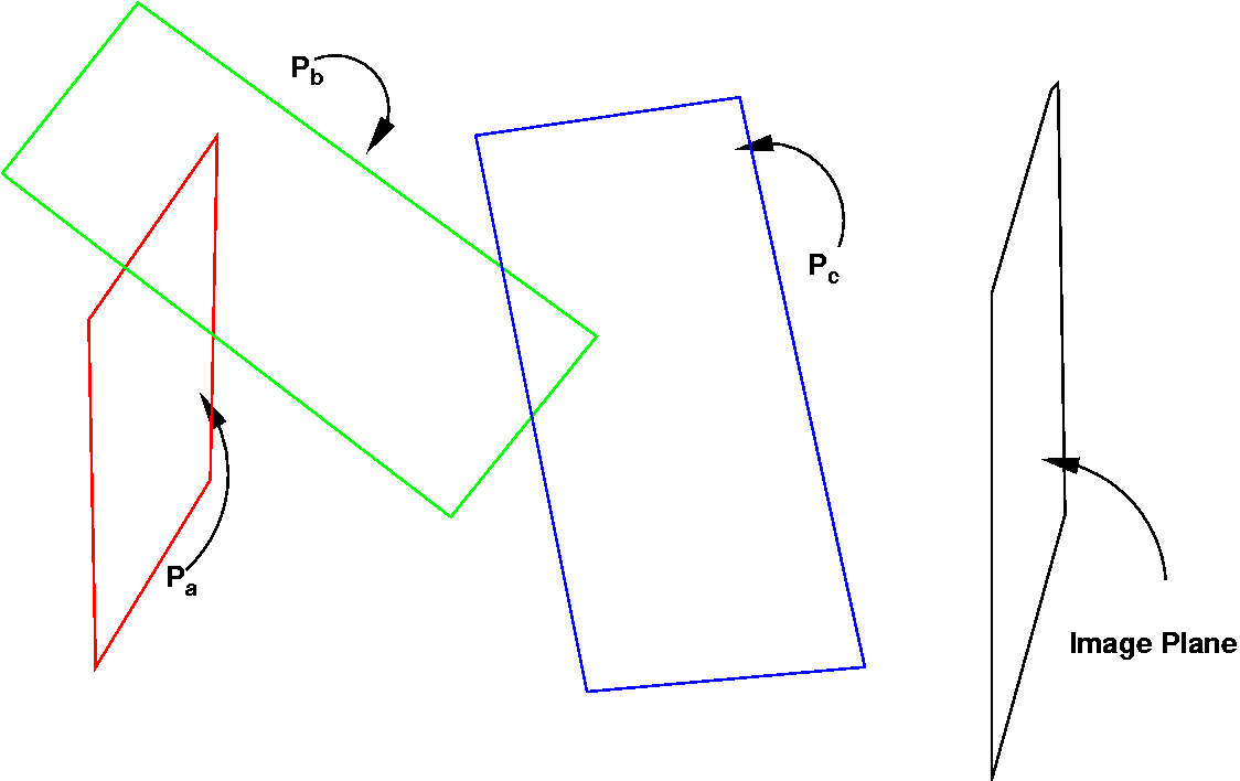
In the above figure we
see a few randomly oriented planes (P a ,Pb
, Pc ) which donot intesect each other in the middle
and which are to be imaged orthographically onto the image plane. Here
the planes are such that,
w.r.t the image plane, Pc lies infront of both the planes completely while a portion of Pb lies behind P a and portion of it lies in front. I hope you get the picture. In figure Fig (2) we see what the projections of these planes on the image plane look like.
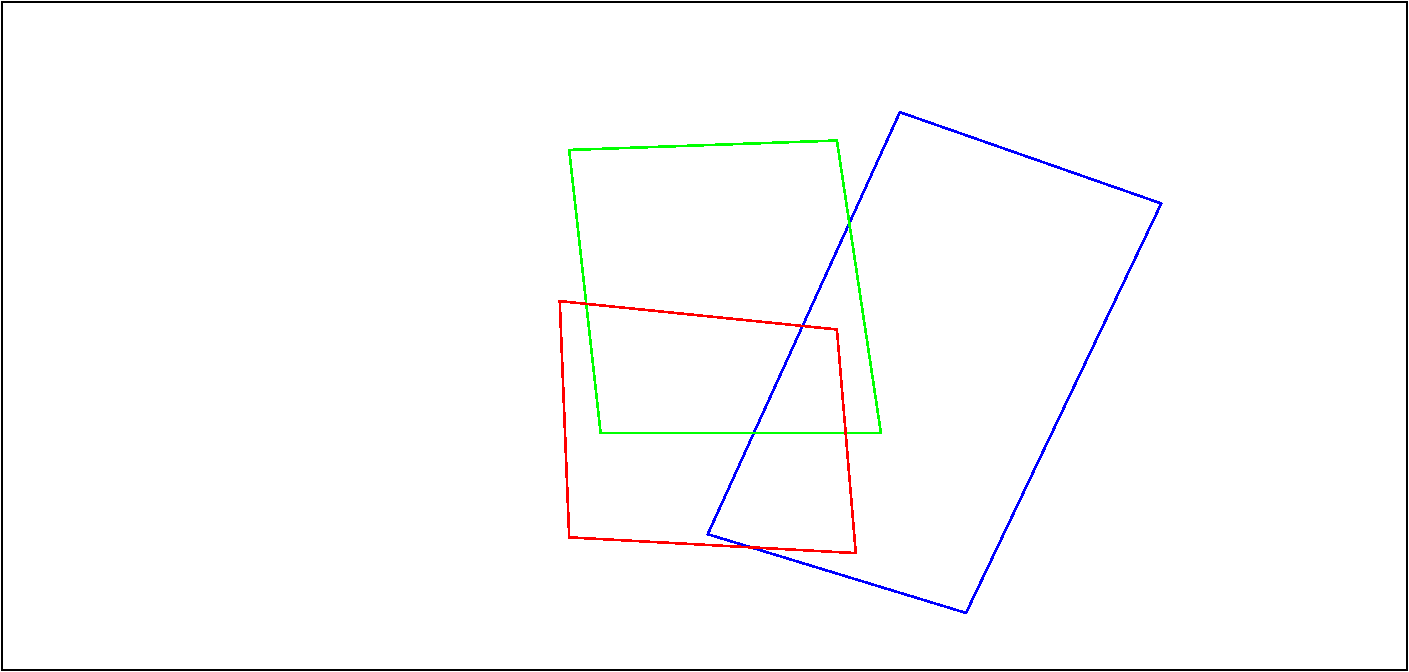
Polygons which are projections of the planes in the 3D world onto the image plane
Fig (2)
The colour codes will help you to identify the planes from Fig (1). Note here we have drawn all the lines in bold. What we want to do is to draw the hidden lines (or parts of lines) as dotted. So that the figure should look somewhat like in Figure (3).
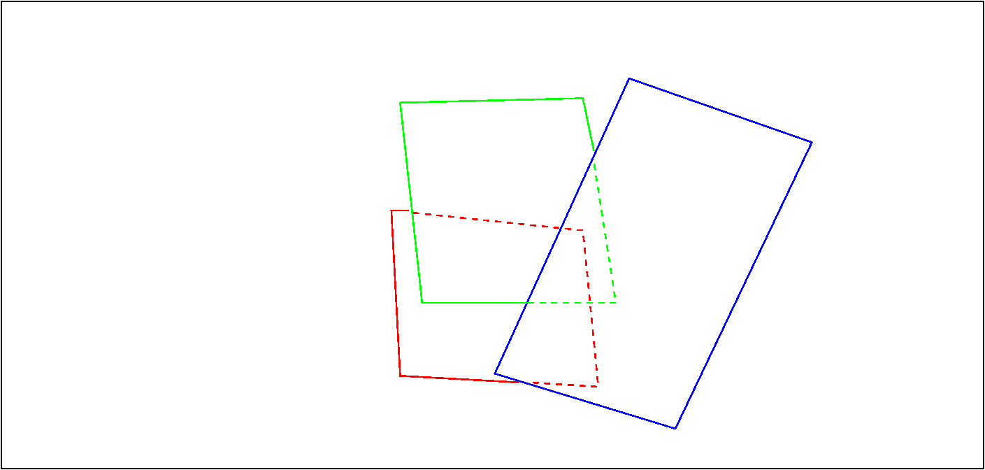
The desired output image.
Fig (3)
Let us see how we can achieve this. We now make a justified observation that a dotted line drawn on top of a solid one does not make any difference. Infact this is the idea that we borrowed from some of your classmates scheme. (Of course we believe that we are drawing all the edges in the same colour).
Let us now proceed to the algorithm.
We assume that we have computed the projected polygons, the one's shown in Figure Fig (2), and have stored them in an array, call it Arr_A of polygons, in no particular order. However we maintain the information which polygon in Fig (2) is associated with which plane in the 3D world. We have two more arrays of polygons which are initially empty, let us call them Arr_B and Arr_C. We will ultimately render the polygons in Arr_B and Arr_C and we do so only when Arr_A becomes empty. At any stage of the algorithm we do the following.
We pick up the next polygon Pj from Arr_A and do the following.
For all polygons Pi belonging to Arr_B do
compute the polygon Pk = Pj¤ Pi
If Pk not null
consider a point q within Pk and determine its corresponding points Qi and Qj on the 3D
planes corresponding to Pi and Pj respectively.
if Qi is closer to the image plane then set Pj = Pj - Pi and add Pk to Arr_C.
else Qj is closer to the image plane and thus replace Pi = Pi - Pj in Arr_B and add Pk to Arr_C.
When all polygons Pi belonging to Arr_B has been checked with Pj add Pj to Arr_B.
When Arr_A is exhausted then render all the polygons in Arr_B with solid lines and all those in Arr_C with dotted lines.
It seems to us that the above algorithm will work, Here we run the algorithm on the situation depicted in Fig(1).
The different stages of the algorithm are shown below.
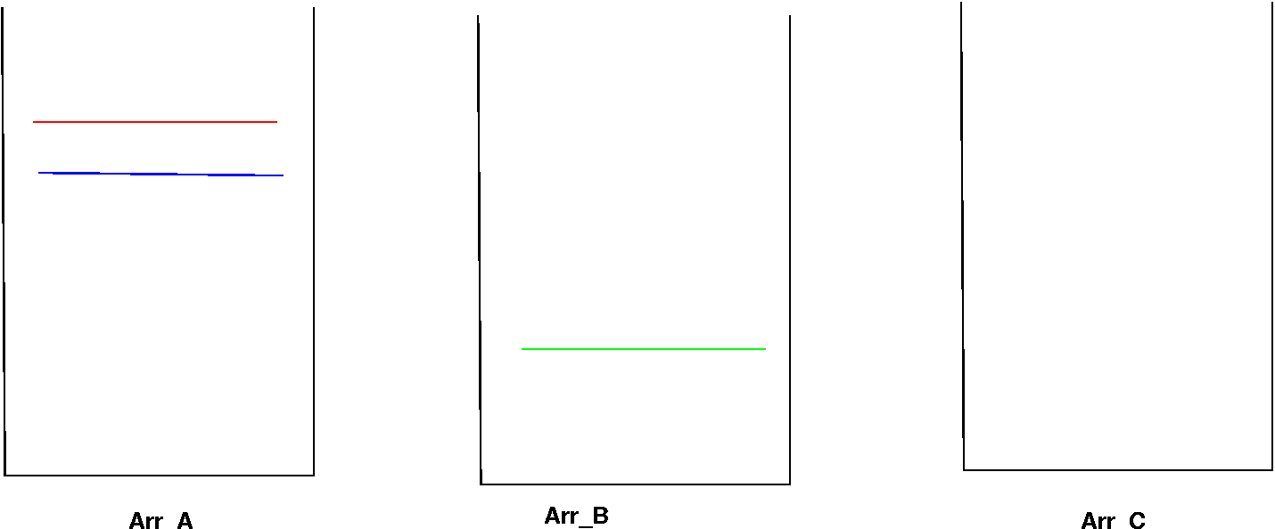
Stage(1)
Arr_A has all the three projected polygons Arr_B and Arr_C are empty.
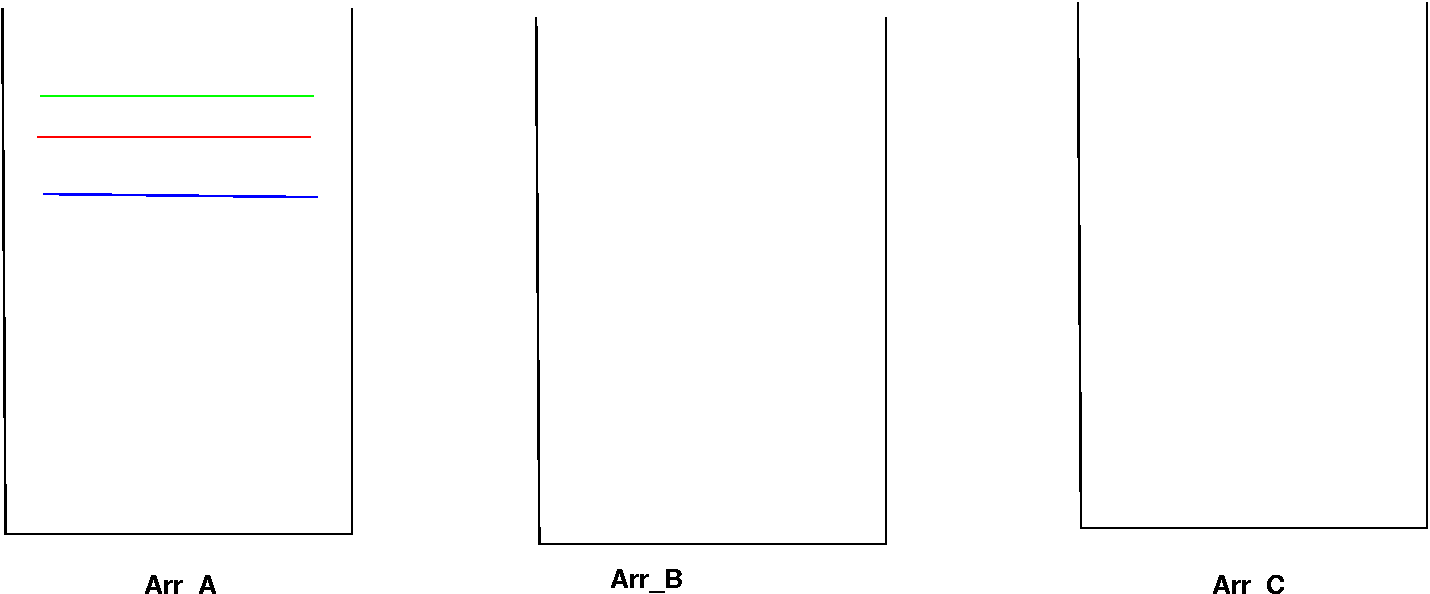
Stage(2)
Arr_A has two projected polygons Arr_B has 1 and Arr_C is empty. Here the green polygon was not tested with any other polygon (see algo above) as Arr_B was empty.
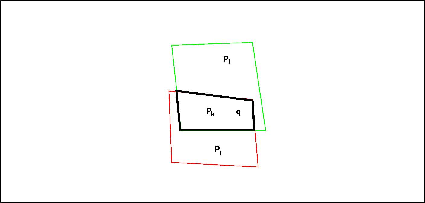
Stage(3)
The red polygon is picked from Arr_A and this becomes our Pj and is tested with the only polygon in Arr_B which is the green polygon, thus the green polygon is Pi . The intersection polygon Pk is indicated as the black polygon. The point q is considered inside Pk and it is found that at this point Pi (green) is closer to the image plane than Pj (red). We thus add Pk to Arr_C and replace the red polygon Pj by the polygon Pj-Pi . As there are no more polygons in Arr_B to test Pj with, we add Pj to Arr_B .
w.r.t the image plane, Pc lies infront of both the planes completely while a portion of Pb lies behind P a and portion of it lies in front. I hope you get the picture. In figure Fig (2) we see what the projections of these planes on the image plane look like.
Polygons which are projections of the planes in the 3D world onto the image plane
Fig (2)
The colour codes will help you to identify the planes from Fig (1). Note here we have drawn all the lines in bold. What we want to do is to draw the hidden lines (or parts of lines) as dotted. So that the figure should look somewhat like in Figure (3).
The desired output image.
Fig (3)
Let us see how we can achieve this. We now make a justified observation that a dotted line drawn on top of a solid one does not make any difference. Infact this is the idea that we borrowed from some of your classmates scheme. (Of course we believe that we are drawing all the edges in the same colour).
Let us now proceed to the algorithm.
We assume that we have computed the projected polygons, the one's shown in Figure Fig (2), and have stored them in an array, call it Arr_A of polygons, in no particular order. However we maintain the information which polygon in Fig (2) is associated with which plane in the 3D world. We have two more arrays of polygons which are initially empty, let us call them Arr_B and Arr_C. We will ultimately render the polygons in Arr_B and Arr_C and we do so only when Arr_A becomes empty. At any stage of the algorithm we do the following.
We pick up the next polygon Pj from Arr_A and do the following.
For all polygons Pi belonging to Arr_B do
compute the polygon Pk = Pj¤ Pi
If Pk not null
consider a point q within Pk and determine its corresponding points Qi and Qj on the 3D
planes corresponding to Pi and Pj respectively.
if Qi is closer to the image plane then set Pj = Pj - Pi and add Pk to Arr_C.
else Qj is closer to the image plane and thus replace Pi = Pi - Pj in Arr_B and add Pk to Arr_C.
When all polygons Pi belonging to Arr_B has been checked with Pj add Pj to Arr_B.
When Arr_A is exhausted then render all the polygons in Arr_B with solid lines and all those in Arr_C with dotted lines.
It seems to us that the above algorithm will work, Here we run the algorithm on the situation depicted in Fig(1).
The different stages of the algorithm are shown below.
Stage(1)
Arr_A has all the three projected polygons Arr_B and Arr_C are empty.
Stage(2)
Arr_A has two projected polygons Arr_B has 1 and Arr_C is empty. Here the green polygon was not tested with any other polygon (see algo above) as Arr_B was empty.
Stage(3)
The red polygon is picked from Arr_A and this becomes our Pj and is tested with the only polygon in Arr_B which is the green polygon, thus the green polygon is Pi . The intersection polygon Pk is indicated as the black polygon. The point q is considered inside Pk and it is found that at this point Pi (green) is closer to the image plane than Pj (red). We thus add Pk to Arr_C and replace the red polygon Pj by the polygon Pj-Pi . As there are no more polygons in Arr_B to test Pj with, we add Pj to Arr_B .
The figure below shows the state of the three arrays after this stage. Note that the polygons in Arr_B (the red and green ones are disjoint polygons).

Stage(4)
The last blue polygon is picked from Arr_A and this becomes our Pj and is tested with the two polygons in Arr_B which are the read and green polygons, Firstly the test is with the red polygon (actually the portion of the red polygon left from the previous stage). It results in the following.
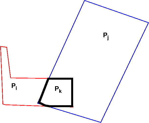
What results is that the Pk shown in black is added to Arr_C . The depth test described in the algorithm for a point in Pk results the polygon Pi to be eaten away further. The blue polygon remains as it is and is further tested with the green polygon. Actually you should start to see how the algorithm works by now. Anyways you can work out the remaining steps. Thus in the end. The polygons in Arr_B are rendered solid and those in Arr_C are rendered as dashed lines.
We are doing about O(n^2) polygon operations if there are n polygons. The actual complexity (in the worst case sense) in terms of the number of edges can be worked out utilising Euler’s theorem.
Just think about this scheme and post your comments in the mailing list.