Consider an ordinary differential equation of the form
We need to solve this equation and obtain the value of the function ![]() at some point
at some point ![]() . For any value
. For any value ![]() and a small step
and a small step ![]() we have
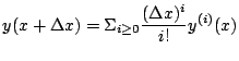
from the Taylor series expansion
we have
from the Taylor series expansion
where
![]() denotes the
denotes the ![]() -th total derivative of
-th total derivative of ![]() at the point
at the point
![]() . By truncating the Taylor
expansion upto some value
. By truncating the Taylor
expansion upto some value ![]() we could get
fairly close to the actual solution of equation (1). However, this
requires being able to find derivatives upto order
we could get
fairly close to the actual solution of equation (1). However, this
requires being able to find derivatives upto order ![]() . That is usually
very difficult and time-consuming for arbitrary functions.
. That is usually
very difficult and time-consuming for arbitrary functions.
A fairly accurate method for obtaining numerical solutions to equation (1) is the Runge-Kutta method1 and is used in most packages. In this method there is no need to calculate higher order derivatives.
Runge-Kutta Methods
We describe below the Runge-Kutta method of second order:
Let the interval
![]() be divided into steps of size
be divided into steps of size
![]() , for some appropriately chosen
, for some appropriately chosen ![]() .
Assume we want to to compute
.
Assume we want to to compute
![]() using a formula of the
form of the form
using a formula of the
form of the form
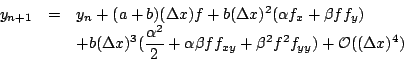
On expanding
![]() through the Taylor expansion we get
through the Taylor expansion we get
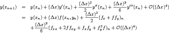
On the other hand using Taylor's exapansion for functions of two variables we get that
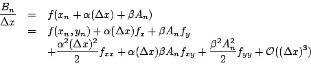
If we substitute this expression for ![]() into the formula (3)
and use
into the formula (3)
and use
![]() , we find after rearranging the powers of
, we find after rearranging the powers of
![]() that
that
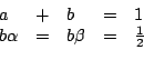
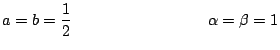
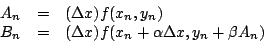
As one can see it is not necessary to compute any higher derivatives, yet it is possible to get an accuracy upto the second-order terms of the Taylor expansion. Hence this method is called Runge-Kutta of second order. An even more accurate method called the Runge-Kutta of fourth order involves computing four auxiliary quantities
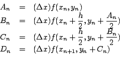
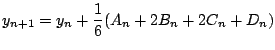
and using the formula
This method can be shown to be accurate upto the fourth order terms of the Taylor expansion. However it is too complicated and tedious to explain and justify.
What you have to do
Develop a higher order function runge_kutta_4 which solves any ordinary
initial value problem for a given parameter ![]() using the fourth order
Runge-Kutta method (4). Give at least 5 examples
of functions involving trigonometric functions, exponentials and polynomials
and setup initial value problems and solve them for chosen values of
using the fourth order
Runge-Kutta method (4). Give at least 5 examples
of functions involving trigonometric functions, exponentials and polynomials
and setup initial value problems and solve them for chosen values of ![]() and
determine the extent to which the anlytical solutions match the numerical solutions.
Note:
and
determine the extent to which the anlytical solutions match the numerical solutions.
Note: