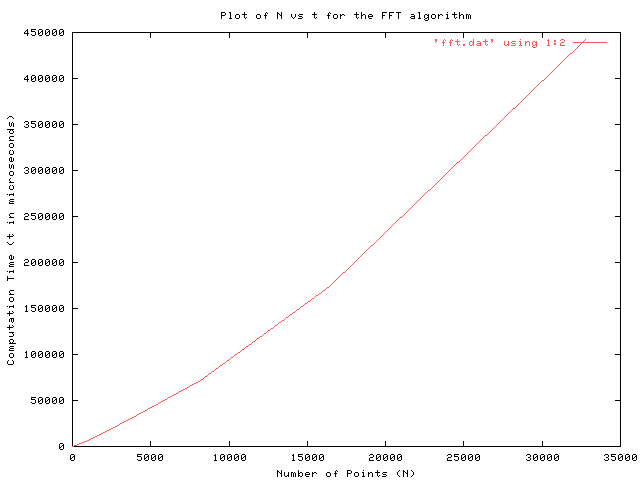
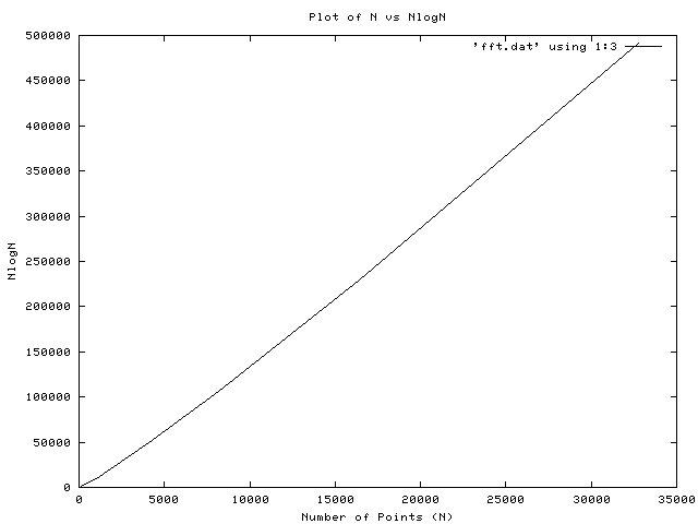
These plot actually help us charecterize the order
of the Fast Fourier Transform Algorithm. Comparing the plot of Computation
Time `t' (in microseconds) vs N to the plot of NlogN
vs N, it can be seen that they show identical growth behaviour. At any
value
of N , t can shown to bounded by cNlogN where c may
be any arbitrary constants.
Method of data collection -
1. A complex array was filled with `N'
elements (values randomly varying between 0 to 1) . Then the `gettimeofday()'
system call
was used to record time
before calling the FFT calculating function with the complex array, and
again the time was recorded
after returning from the
function.
2. These values (the values of `N' and the time taken) were recorded onto a data file and were plotted as shown below.
3. Then this was repeated for other values
of `N', increasing `N' through a loop from 22 to 215,
and getting the corresponding
times.
I repeated this process several times to see the behaviour
of the time values as sampling by this method induces errors in
a multiprocess environment such as Linux, but the
variation was small at the microsecond level as the tests were done
on a single user machine.
Profiling was not done because gprof takes a sample
0.01 seconds so it only gives non-zero times for arrays with size greater
than 212. Valid profiling data obtained
is given at the end of this page.
The Data Table
|
|
|
|
|
|
|
|
|
|
|
|
|
|
|
|
|
|
|
|
|
|
|
|
|
|
|
|
|
|
|
|
|
|
|
|
|
|
|
|
|
|
|
|
|
|
|
|
|
|
|
|
|
|
|
|
|
|
|
|
|
|
|
|
The Plots
|
|
Profiling Data collected -
|
|
|
|
|
|
|
|
|
|
|
|
|
|
|
| Page last updated on 28 January, 2004. |
 AT cse.iitd.ac.in AT cse.iitd.ac.in
|
© Parag Chaudhuri , 2009 |

|

|

|
|
|