|
SOLUTION OF SYSTEM OF LINEAR EQUATIONS USING
JACOBI METHOD
BACKGROUND The system of linear equations [A]{x} = {b} is given byCONJUGATE GRADIENT METHOD BACKGROUND Iterative methods are techniques to solve systems of equations of the form [A]{x}={b} that generate a sequence of approximations to the solution vector x. In each iteration, the coefficient matrix A is used to perform a matrix-vector multiplication. The number of iterations required to solve a system of equations depends on input data matrix and hence, the number of iterations is not known prior to executing the algorithm. Iterative methods do not guarantee a solution for all systems of equations. However, when they do yield a solution, they are usually less expensive than direct methods for matrix factorization for large matrix system of equations.SOLUTION OF SYSTEM OF LINEAR EQUATIONS USING GAUSSIAN ELIMINATION METHOD BACKGROUND The system of linear equations [A]{x} = {b} is given bySPARSE MATRIX COMPUTATION BACKGROUND We can classify matrices into two broad categories according to the kind of algorithms that are appropriate for them. The first category is dense or full matrices with few or no zero entries. The second category is sparse matrices in which a majority of the entries are zero. In order to process a matrix input in parallel, we must partition it so that the partitions can be assigned to different processes. The computation and communication performed by all the message-passing programs presented so far (matrix vector and matrix-matrix algorithms for dense matrices) are quite structured. In particular, every process knows with which process it needs to communicate and what data it needs to send and receive . This is evident from matrix-matrix multiplication and matrix-vector multiplication algorithms. This information is used to map the computation onto the parallel computer and to program the required data transfers. However, there are problems in which we cannot determine a priori the processes that needs to communicate and what data they need to transfer. These problems often involve operations on irregular grid or unstructured data. Also, the exact communication patterns are specific to each particular problem and it may vary from problem to problem. Sparse matrix into vector requires unstructured communication.SAMPLE SORT BACKGROUND Sorting is defined as the task of arranging an unordered collection of elements into monotonically increasing (or decreasing) order. Specifically, let S =(a1, a2,........, an) be a sequence of n elements in an arbitrary order; sorting transforms S into a monotonically increasing sequence S* = (a1*, a2* ,........, an*), such that ai*<= aj* for 1<=i<=j<=n, and S * is a permutation of S . Parallelizing a sequential sorting algorithm involves distributing the elements to be sorted onto the available processes. This procedure raises a number of issues such as where the input and output sequences are stored and How comparisons are performed ?. One has to address in order to make the presentation of parallel sorting algorithms effectively. SOLUTION OF PARTIAL DIFFERENTIAL EQUATIONS BY FINITE DIFFERENCE METHODBACKGROUNDA significant number of the application problems in the various scientific fields involve the solution of coupled partial differential equation (PDE) systems in complex geometries. Finite Difference (FD) methods have been used to solve the coupled PDE systems. The first step in the solution process is to generate structured or unstructured grid in the given domain. The second step is to obtain the numerical approximations to the derivatives and unknown functions in PDE at each grid point and formulate the matrix system of linear equations. The last step is to solve the matrix system of equations after imposing boundary conditions. In the FD method, the entities within the grid elements are simulated with respect to the influence of the other entities and their surroundings. Since many such systems are evolving with time, time forms an additional dimension for these computations. Even for a small number of grid points, a three dimensional coordinate system, and a reasonable discritized time step, most of the models involve trillions of operations.
Write a parallel MPI program, for solving system of linear equations [A]{x} = {b} on a p processor PARAM 10000 using Jacobi method.
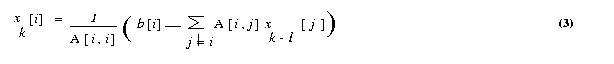
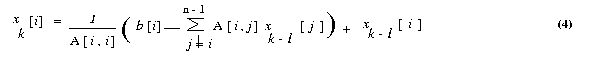
The Jacobi iterative method is one of the simplest iterative techniques. The ith equation of a system of linear equations [A]{x}={b} is 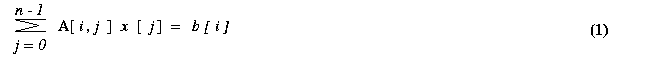 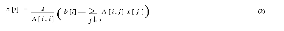
The input should be in following format. Assume that the real matrix is of size m x n and the real vector is of size n . Also the number of rows m should be greater than or equal to number of processes p. Process with rank 0 reads the input matrix A and the vector x . Format for the input files are given below. Input file 1 The input file for the matrix should strictly adhere to the following format. #Line 1 : Number of Rows (m), Number of columns(n).
A sample input file for the matrix (8 x 8) is given below
Input file 2 The input file for the vector should strictly adhere to the following format. #Line 1 : Size of the vector (n)
A sample input file for the vector (8 x 1) is given below 8
Process 0 will print the results of the solution x of matrix/system
Ax = b.
1.0 1.0 1.0 1.0 1.0 1.0 1.0 1.0 
You will implement a simple parallel Conjugate Gradient Method with MPI library to solve the system of linear equations [A]{x}={b}. Assume that A is symmetric positive definite matrix.
The conjugate gradient method The conjugate gradient (CG) method is an example of minimizing
method. A real n x n matrix A is positive definite if xT A
x > {0} for any n x 1 real, nonzero vector x. For a symmetric
positive definite matrix A, the unique vector x that minimizes
the quadratic functional f (x) = (1/2)xTAx-xTb
is the solution to the system Ax = b, here
x and b are n x 1 vectors. It is not particularly relevant
when n is very large, since the conjugating time for that number of iterations
is usually prohibitive and the property does not hold in presence of rounding
errors. The reason is that the gradient of functional f (x) is
Ax - b, which is zero when f (x) is
minimum. The gradient of a function is a n x 1 vector. We explain
some important steps in the algorithm. An iteration of a minimization method
is of the form
tau k = gkTgk / dkTAdk, (2) gk+1 = Axk+1 - b = Axk- b + tauk Adk = gk + tauk Adk (3) 2. xk+1 = xk + tauk dk 3. gk+1 = gk + tauk Adk 4. Betak+1 = gTk+1gk+1/ gTkgk 5. dk+1 = -gk+1 + Betak dk The computer implementation of this algorithm is explained as follows void CongugateGradient(float
x0[ ], float b [ ], float d)
float g, Delta0, Delta1, beta;
iteration = 0;
if ( Delta0 <= EPSILON)
do {
iteration = iteration + 1;
if ( Delta1 <= EPSILON )
beta = Delta1 / Delta0;
} while(Delta0 > EPSILON && Iteration < MAX_ITERATIONS);
return;
Regarding one-dimensional arrays of size n x 1 are required for
temp, g, x, d. The storage requirement for matrix
The speed of convergence of the CG algorithm can be increased by preconditioning A with the congruence transformation A* = E-1AE-T where E is a nonsingular matrix. E is chosen such that A* has fewer distinct eigen values than A. The CG algorithm is then used to solve A* y =b*, where x =(ET)-1y . The resulting algorithm is called the preconditioned conjugate gradient (PCG) algorithm. The step performed in each iteration of the preconditioned conjugate gradient algorithm are as follows 2. xk+1 = xk + tauk dk 3. gk+1 = gk + tauk Adk 4. hk+1 = C-1gk+1 5. betak+1 = gTk+1hk+1/ gTkhk 6. dk+1 = -hk+1 + betak+1dk
The parallel conjugate gradient algorithm involves the following type of computations and communications Partitioning of a matrix : The matrix A is obtained by discretization
of partial differential equations by finite element, or finite difference
method. In such cases, the matrix is either sparse or banded. Consequently,
the partition of the matrix onto p processes play a vital
role for performance. For, simplicity , we assume that A is symmetric
positive definite and is rowwise block-striped partitioned.
Vector inner products :
Matrix-vector multiplication :
Solving the preconditioned system :
The convergence of CG method iterations performed by checking the error criteria i.e. eulicidean norm of the residual vector should be less than prescribed tolerance. This convergence check involves gathering of real value from all processes, which may be very costly operation. We consider parallel implementations of the PCG algorithm using diagonal preconditioner for dense coefficient matrix type. As we will see, if C is a diagonal preconditioner, then solving the modified system does not require any interprocessor communication. Hence, the communication time in a CG iteration with diagonal preconditioning is the same as that in an iteration of the unpreconditioned algorithm. Thus the operations that involve any communication overheads are computation of inner products, matrix-vector multiplication and, in case of IC preconditioner solving the system.
The input should be in following format. Assume that the real matrix is of size m x n and the real vector is of size n . Also the number of rows m should be greater than or equal to number of processes p. Process with rank 0 reads the input matrix A and the vector x . Format for the input files are given below. Input file 1 The input file for the matrix should strictly adhere to the following format. #Line 1 : Number of Rows (m), Number of columns(n).
A sample input file for the matrix (8 x 8) is given below
The input file for the vector should strictly adhere to the following format. #Line 1 : Size of the vector (n)
A sample input file for the vector (8 x 1) is given below
Process 0 will print the results of the solution x of matrix/system Ax = b. 1.0 1.0 1.0 1.0 1.0 1.0 1.0 1.0
linear equations by Gaussian Elimination method
Write a MPI program to solve the system of linear equations [A]{x} = {b} using Gaussian elimination without pivoting and a back-substitution. Assume that A is symmetric positive definite dense matrix of size n. You may assume that n is evenly divisible by p.
The system of linear equations is given by In matrix notation, this system of linear equation is written as [A]{x}={b} where A[i, j] = ai, j , b is an n x 1 vector [bo,b1,...,bn-1]T, and is the desired solution vector [xo,x1,...,xn-1]T. We will make all subsequent references to ai, j by A[i, j] and xi by x[i ]. The matrix A is partitioned using block row-wise striping. Each process has n/p rows of the matrix A and the vector b. Since only process with rank 0 performs input and output, the matrix and vector must be distributed to the other processes.
void
Gaussian_Elimination (float A[ ][ ], float b[ ], float
y[ ], int n)
for (k = 0; k < n; k++)
Program 1 : A serial gaussian elimination algorithm that converts the system
of linear
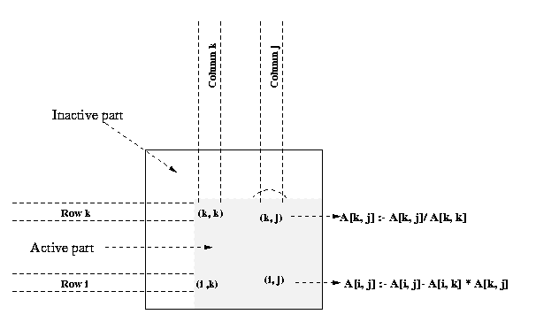
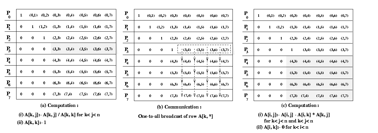
of this section. This program converts a system of linear equations [A]{x}={b} to a unit upper-triangular system [U]{x}={y}. We assume that the matrix U shares storage with A and overwrites the upper-triangular portion of A. The element A[k, j] computed on line 6 of above program is actually U[k, j]. Similarly, the element A[k, k] equated to 1 on line 8 is U[k, k]. The above program assumes that A[k, k] not equal to 0 when it is used as a divisor on lines 6 and 7. A typical computation of Gauss elimination procedure in the kth iteration of the outer loop is shown in the Figure 17
We discuss parallel formulations of the classical Gaussian elimination method for upper-triangularization. We describe a straight-forward Gaussian elimination algorithm assuming that the coefficient matrix is non singular and symmetric positive definite. We consider a parallel implementation of program 1 in which the coefficient matrix is rowwise strip-partitioned among the processes. A parallel implementation of this algorithm with column-wise striping is very similar, and its details can be worked out based on the implementation using rowwise striping.
Figure 18 Gaussian elimination steps during the iteration
corresponding to k = 3 for an 8 X 8 matrix and striped
Figure 18 illustrates the computation and communication that
takes place in the iteration of the outer loop when k = 3. We first
consider the case in which one row is assigned to each process, and the
n x n coefficient matrix A is striped among n processes
labeled from P0 to Pn-1.
In this mapping , process Pi initially stores elements
A[i, j] for
Program 1 and Figure 18 show that A[k, k+1], A[k,
k+2],..., A[k, n-1] are divided by A[k,
k] (line 6) at the beginning of the kth iteration.
All matrix elements participating in this operation lie on the same process
(shown by the shaded portion of the matrix in Figure 18(b). So this step
does not require any communication. In the second computation step of the
algorithm (the elimination step of line 12), the modified (after division)
elements of the kth row are used by all other rows of
the active part of the kth row to the processes storing
rows k+1 to n-1. Finally, the computation
This example was chosen not because it illustrates the best way to parallelize this particular numerical computation (it doesn't), because it illustrates the basic MPI send and receive operations in the context of fundamental type of parallel algorithm, applicable in many situations.
The input should be in following format. Assume that the real matrix is of size m x n and the real vector is of size n . Also the number of rows m should be greater than or equal to number of processes p. Process with rank 0 reads the input matrix A and the vector x . Format for the input files are given below. Input file 1 The input file for the matrix should strictly adhere to the following format. #Line 1 : Number of Rows (m), Number of columns(n).
A sample input file for the matrix (8 x 8) is given below
Input file 2 The input file for the vector should strictly adhere to the following format. #Line 1 : Size of the vector (n)
A sample input file for the vector (8 x 1) is given below
Process 0 will print the results of the solution x of matrix/system Ax = b. 1.0 1.0 1.0 1.0 1.0 1.0 1.0 1.0 using block-striped partitioning
Write a MPI program on sparse matrix multiplication of size n x n and vector of size n on p processors of PARAM 10000. Assume that n is evenly divisible by p .
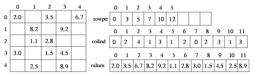
Dense matrices are stored in the computer memory by using two-dimensional arrays. For example, a matrix with n rows and m columns, is stored using a n x m array of real numbers. However, using the same two-dimensional array to store sparse matrices has two very important drawbacks. First, since most of the entries in the sparse matrix are zero, this storage scheme wastes a lot of memory. Second, computations involving sparse matrices often need to operate only on the non-zero entries of the matrix. Use of dense storage format makes it harder to locate these non-zero entries. For these reasons sparse matrices are stored using different data structures. The Compressed Storage format (CSR) is a widely used scheme for storing sparse matrices. In the CSR format, a sparse matrix A with n rows having k non-zero entries is stored using three arrays: two integer arrays rowptr and colind, and one array of real entries values. The array rowptr is of size n+1, and the other two arrays are each of size k. The array colind stores the column indices of the non-zero entries in A, and the array values stores the corresponding non-zero entries. In particular, the array colind stores the column-indices of the first row followed by the column-indices of the second row followed by the column-indices of the third row, and so on. The array rowptr is used to determine where the storage of the different rows starts and ends in the array colind and values. In particular, the column-indices of row i are stored starting at colind [rowptr[i] ] and ending at (but not including) colind [rowptr[i+1] ]. Similarly, the values of the non-zero entries of row i are stored at values [rowptr[i] ] and ending at (but not including) values [rowptr[i+1] ]. Also note that the number of non-zero entries of row i s simply rowptr[i+1]-rowptr[i].
Figure 19 CSR format of a sample matrix
The following function performs a sparse matrix-vector multiplication
[y]={A} {b} where the sparse matrix A is of size n x m,
the vector b is of size m and the vector y is of size
n. Note that the number of columns of A (i.e., m )
is not explicitly specified as part of the input unless it is required.
int i, j;}
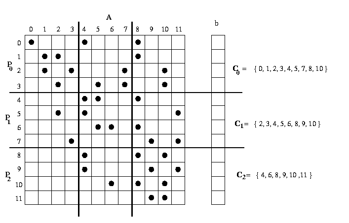
Consider the problem of computing the sparse matrix-vector product [y] = {A}{b} where A is a sparse matrix of size m x n and b is a dense vector using block striped partitioning. In the block striped partitioning of a matrix, the matrix is divided into groups of complete rows or columns, and each process is assigned one such group.
Figure 20 The data needed by each processor in order to compute the sparse matrix-vector product In Figure 20, a sparse matrix A and the corresponding vector b are distributed among three processors. Note that processor po needs to receive elements {4,5,7} from processor p1 and elements {8,10} from processor p2 . However, processor p2 needs to receive only elements {4,6} from processor p1. The process p1 needs to receive elements {2,3} from process p0 and elements {8,9,11} from process p2. Since the exact position of the non-zeros in A is not known a priori, and is usually different for different sparse matrices, we can not write a message-passing program that performs the required data transfers by simply hard coding. The required communication patterns may be different for different processes. That is, one process may need to receive some data from just a few processes whereas another process may need to receive data from almost all processes. The present algorithm partitions the rows of matrix A using block-striped partitioning and the corresponding entries of vector b among the processes, so that each of the p processes gets m/p rows of the matrix and n/p elements of the vector. The portion of the matrix A obtained by block-striped partitioning, is assigned to each process and the non-zero entries of the sparse matrix A is stored using the compressed storage (CSR) format in the arrays rowptr, colind and values. To obtain the entire vector on all processes, MPI_Allgather collective communication is performed. Each process now is responsible for computing the elements of the vector y that correspond to the rows of the matrix that it stores locally. This can be done as soon as each process receives the elements of the vector b that are required in order to compute these serial sparse dot-products. This set of b elements depends on the position of the non-zeros in the rows of A assigned to each process. In particular, for each process pi, let Ci be the set of column-indices j that contain non-zero entries overall the rows assigned to this process. Then process pi needs to receive all the entries of the form bj for all j in Ci . It is a simple parallel program but inefficient way of solving this problem because to write a message-passing program in which all the processes receive the entire b vector. If each row in the matrix has on the average d non-zero entries, then each process spends (md/p) time in serial algorithm. The program will achieve meaningful speedup only d >= p . That is, the number of non-zero entries at each row must be at least as many as the number of processes. This scheme performs well when the sparse matrices are relatively dense. However, in most interesting applications, the number of non-zero entries per row is small, often in the range of 5 to 50. In such cases, the algorithm spends more communication time relative to computation.
One can design efficient algorithm by reducing communication cost by storing the necessary entries of the vector b . In the above algorithm, the overall communication performed by each process can be reduced if each process receives from other processes only those entries of the vector b are needed. In this case, we further reduce the communication cost by assigning only rows of the sparse matrix to processes such that the number of rows required but remotely stored entries of the vector b is minimized. This can be achieved by performing a min-cut partitioning of the graph that corresponds to the sparse matrix. We first construct graph corresponds to sparse matrix and the graph is partitioned among p processes. The off process communication is developed to identify the required values of the vector b residing on neighbouring processes.
The input is available in following format. Assume that the sparse square matrix is of size n and is divisible by the number of processes p . Assume that the vector is of size n. For convenience, the sparsity is defined as maximum non-zero elements in a row, over all the rows. In the given example sparsity is 4. All the entries in the sparse matrix are floating point numbers. Process 0 reads the data. You have to adhere strictly the following format for the input files. Input file 1 # Line 1 : (Sparsity value)
A sample input file for the sparse matrix of size 16 x 16 is given below
:
Input file 2 # Line 1 : (Size of the vector)
A sample input file for the sparse vector of size 16 is given below
:
Process with rank 0 prints the final sparse matrix-vector product.
Write a MPI program to sort n integers, using sample sort algorithm on a p processor of PARAM 10000. Assume n is multiple of p.
There are many sorting algorithms which can be parallelised on various architectures. Some sorting algorithms (bitonic sort, bubble sort, odd-even transposition algorithm, shellsort, quicksort) are based on compare-exchange operations. There are other sorting algorithms such as enumeration sort, bucket sort, sample sort that are important both practically and theoretically. First, we explain bucket sort algorithm and we use concepts of bucket sort in sample sort algorithm.
Bucket sort assumes that n elements to be sorted are uniformly distributed over an interval (a, b). This algorithm is usually called bucket sort and operates as below. The interval (a,b) is divided into m equal sized subintervals referred to as buckets . Each element is placed in the appropriate bucket. Since the n elements are uniformly distributed over the interval (a,b), the number of elements in each bucket is roughly n/m. The algorithm then sorts the elements in each buckets, yielding a sorted sequence. Parallelizing bucket sort is straightforward. Let n be the number of elements to be sorted and p be the number of processes. Initially, each process is assigned a block of n/p elements, and the number of buckets is selected to be m=p. The parallel formulation of bucket sort consists of three steps. In the first step, each process partitions its block of n/p elements into p subblocks on for each of the p buckets. This is possible because each process knows the interval [a,b] and thus the interval for each bucket. In the second step, each process sends subblocks to the appropriate processes. After this step, each process has only the elements belonging to the bucket assigned to it. In the third step, each process sorts its bucket internally by using an optimal sequential sorting algorithm. The performance of bucket sort is better than most of the algorithms and it is a good choice if input elements are uniformly distributed over a known interval.
Sample sort algorithm is an improvement over the basic bucket sort algorithm. The bucket sort algorithm presented above requires the input to be uniformly distributed over an interval [a,b]. However, in many cases, the input may not have such a distribution or its distribution may be unknown. Thus, using bucket sort may result in buckets that have a significantly different number of elements, thereby degrading performance. In such situations, an algorithm called sample sort will yield significantly better performance. The idea behind sample sort is simple. A sample of size s is selected from the n-element sequence, and the range of the buckets is determined by sorting the sample and choosing m-1 elements from the results. These elements (called splitters) divide the sample into m equal sized buckets. After defining the buckets, the algorithm proceeds in the same way as bucket sort . The performance of sample sort depends on the sample size s and the way it is selected from the n-element sequence. How can we parallelize the splitter selection scheme? Let p be the number of processes. As in bucket sort , set m =p; thus, at the end of the algorithm, each process contains only the elements belonging to a single bucket. Each process is assigned a block of n/p elements, which it sorts sequentially. It then chooses p-1 evenly spaced elements from the sorted block. Each process sends its p-1 sample elements to one process say Po. Process Po then sequentially sorts the p(p-1) sample elements and selects the p-1 splitters. Finally, process Po broadcasts the p-1 splitters to all the other processes. Now the algorithm proceeds in a manner identical to that of bucket sort . The sample sort algorithm has got three main phases. These are: 1. Partitioning of the input data and local sort :
2. Choosing the Splitters :
3.Completing the sort :
Process with rank 0 generates unsorted integers using C library call rand().
Process with rank 0 stores the sorted elements in the file sorted_data_out.
by finite difference method
Write a MPI program to solve the Poisson equation with Dirichlet boundary conditions in two space dimensions by finite difference method on structured rectangular type of grid. Use Jacobi iteration method to solve the discretized equations.
In the Poisson problem, the FD method is imposed a regular grid on the physical domain. It then approximate the derivative of unknown quantity u at a grid point by the ratio of the difference in u at two adjacent grid points to the distance between the grid point. In a simple situation, consider a square domain discretized by n x n grid points, as shown in the Figure 21(a). Assume that the grid points are numbered in a row-major order fashion from left to right and from top to bottom, as shown in the Figure 21(b). This ordering is called natural ordering . Given a total of n2 points in the domain n x n grid, this numbering scheme labels the immediate neighbors of point i on the top, left, right, and bottom point as i - n, i -1, i +1 and i+n , respectively. Figure 21(b) represents partitioning of mesh using one dimensional partitioning. 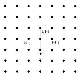 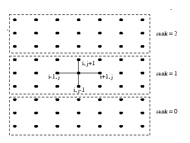
for 2-D problem, with n=7 of Poisson Finite Difference Grid Formulation of Poisson Problem The Poisson problem is expressed by the equations Lu = f(x, y) in the interior of domain [0,1] x [0,1] Where L is Laplacian operator in two space dimensions. u(x,y) = g(x,y) on the boundary of the domain [0,1] x [0,1] We define a square mesh (also called a grid) consisting of the points (xi , yi), given by xi = i / n+1, i=0, ..., n+1, yj = j / n+1, j=0, ..., n+1, where there are n+2 points along each edge of the mesh. We will find an approximation to u(x , y) only at the points (xi, yj). Let ui, j be the approximate solution to u at (xi, yj). and let h = 1/(n+1). Now, we can approximate at each of these points with the formula (ui-1, j +ui, j+1+ui, j-1+ui+1, j-4ui, j )/ h2 = fi, j . Rewriting the above equation as ui, j = 1/4(ui-1, j+ui, j+1+ui, j-1+ui+1, j-h2fi, j), Now jacobi iteration method is employed to obtain final solution starting with initial guess solution ui,jk for k=0 for all mesh points u i,j and solve the following equation iteratively until the solution is converged. ui, jk+1 = 1/4(ui-1, jk+ui, j+1k+ui, j-1k+ui+1, jk-h2fi, j). The resultant discretized banded matrix is shown in the Figure 20
To parallelize this algorithm, the physical domain is sliced into slabs, with the computations on each slab being handled by a different process. We have used block row-wise strip partitioning as shown in Figure 21(a). Each process gets its own partition as shown in the Figure 21(b). To perform the computation in each partition, we need to obtain the grid point information from adjacent processs to compute the values ui,jk for iteration k for all mesh points ui,j near to the partition boundary. The elements of the array that are used to hold data from other processes are called ghost points.
In simple situation, each process sends data to the process on top and then receives data from the process below it. The order is then reversed, and data is sent to the process below and received from the process above. This strategy is simple, it is not necessarily the best way to implement the exchange of ghost points. MPI topologies can be used to create the position of processes and determine the decomposition of the arrays. MPI allows the user to define a particular application, or virtual topology. An important virtual topology is the Cartesian topology. This simply a decomposition in the natural co-ordinate (e.g.. x,y,z) directions. In the implementation of this algorithm, row and column MPI communicators are created. The iteration is terminated when the difference between successive computed solution at all grid points is strictly less than prescribed tolerance. The routine MPI_Allreduce is used to ensure that all processes compute the same value for the difference in all of the elements.
The parallel algorithm used in this model is not efficient and may give poor performance relative to more recent and sophisticated, freely available parallel solver for PDE's that use MPI. This example was chosen not because it illustrates the best way to parallelize this particular numerical computation (it doesn't), because it illustrates the basic MPI send and receive operations, MPI topologies in the context of fundamental type of parallel algorithm, applicable in many situations.
User defines the total number of mesh points along each side of the square mesh (also called as grid) and number of iterations for the convergence of the method on command line. There are n+2 grid points on each side of the square mesh. Process with rank 0 performs all the input such as grid point neighbors, co-ordinate values of the nodes, and number of boundary nodes, Dirichlet boundary condition information on boundary nodes, initial guess solution on process with rank 0 is given. The program automatically generates all necessary input data and the user has to specify total number of grid points. To make the program as simple as possible to follow, error conditions are not checked in MPI library calls. In general one should check these, and if the calls fails, the program needs to exist smoothly. Various special MPI library calls can be used for the solution of poission equation by finite difference method. MPI provides to the programmer, good choice of decomposition depends on the details of the underlying hardware. MPI allows the user to define a particular application, or virtual topology. An important virtual topology is the cartesian topology which is simply a decompostion of a grid. Advanced point-to-point communication library calls such as MPI_Send and MPI_Recv (blocking communication calls), MPI_Send and MPI_Recv ( ordered send and receive blocking communication calls), MPI_SENDRECV ( Combined send and receive), MPI_BSEND (Buffer send), MPI_ISEND, MPI_IRECV (Non-blocking communication calls) and MPI_Ssend (synchronus sends) can be used in the implementation of parallel programe on PARAM 10000. One dimensional and two dimensional decomposition of mesh is used. Jacobi iterative method is employed for the iterative method.
One Dimensional Decomposition of Mesh We consider square grid in a two dimensional region and assume that number of grid points in x-direction and y-direction is same. The actual message passing in our program is carried out by the MPI functions MPI_Send and MPI_Recv. The first command sends a message to a designated process. The second receives a message from a process. We have used simple MPI point-to-point communication calls MPI_Send and MPI_Recv in various programs. We study more detail about the advanced point-to-point communication library calls below. Consider an example in which process 0 wants to send a message to process
1, and there is some type of physical connection between 0 and 1. The message
envelope contains at least the information such as the rank of the
receiver, the rank of the sender, a tag and a communicator. A couple of
natural questions might occur. What if a process one is not ready to receive
it? What can process zero do? There are three possibilities.
As long as there is space available to hold a copy of the message, the message passing system should provide this service to the programmer rather than making the process to stop dead in its tracks until the matching receive is called. Also, there is no information specifying where the receiving processes should store the message. Thus, until process 1 calls MPI_Recv, the system doesn't know where the data that Process 0 is sending should be stored. When Process 1 calls MPI_Recv, the system software that executes receive can see which (if any) buffered message has an envelope that matches the parameters specified by MPI_Recv. If there isn't a message, it waits until one arrives. If the MPI implementation does copy the send buffer into internal storage, we say that it buffers the data. Different buffering strategies provide different levels of convenience and performance. For large applications that are already using a large amount of memory, even requiring the message-passing system to use all available memory may not provide enough memory to make this code work. Sometimes, the code runs (it does not deadlock) but it does not execute in parallel. All of these issues suggest that programmers should be aware of the pitfalls in assuming that the system will provide adequate buffering. If a system has no buffering, then Process 0 cannot send its data until it knows that Process 1 is ready to receive the message, and consequently memory is available for the data. Programming under the assumption that a system has buffering is very common (most systems automatically provide some buffering), although in MPI parlance, it is unsafe. This means that if the program is run on a system that does not provide buffering, the program will deadlock. If the system has no buffering, Process 0's first message cannot be received until Process 1 has signaled that it is ready to receive the first send, and Process 1 will hang while it waits for Process 0 to execute the second send. We will describe ways in which the MPI programmer can ensure that the correct parallel execution of a program does not depend on the amount of buffering, if any, provided by the message-passing system. (1) Ordered Send and Receive We discuss issues regarding MPI functions, which fail if there is no
system buffering. We explain the issues regarding unsafe and provide alternative
solutions. First, why are the functions unsafe? Consider the case that
we have two processes similar to what we have given in Table 3.1. Then
where will be a single exchange of data between process 0 and process 1?
If we synchronize the processes before the exchanges we'll have approximately
the following sequence of events:
As explained earlier, if there's no buffering, the MPI_Send will never return. So process 0 will wait in MPI_Send until process 1 calls MPI_Recv. We've encountered this situation and it is called as deadlock. Two options are considered to make them safe either by re-organising the send and receive or let MPI make them safe through use of different MPI library calls. In order to make them safe by reorganizing the sends and receives,
we need to decide who will send first and who will receive first. One of
the easiest ways to correct for a dependence on buffering is to order the
sends and receives so that they are paired up. That is, the sends and receives
are ordered so that if one process is sending to another, the destination
will do receive that matches that send before doing a send of its own.
Now, the ordered sequence of events is listed in the table 3.2
So there may be a delay in the completion of one communication, but the program will complete successfully. (2) Combined Send and Receive The approach of pairing the sends and receives is effective but can be difficult to implement when the arrangement of processes is complex (for example, with an irregular grid). An alternative is to use special MPI calls, not worrying about deadlock from a lack of buffering. A simpler solution is to let MPI take care of the problem. The function MPI_Sendrecv, as its name implies, performs both send and receive, and it organizes them so that even in systems with no buffering the calling program won't deadlock, at least not in the way that the MPI_Send / MPI_Recv implementation deadlocks. The syntax of MPI_Sendrecv is
int MPI_Sendrecv(void* send_buf, int send_count, MPI_Datatype send_type,
int destination, int send_tag, void* recv_buf, int recv_count, int
recv_type, int source, int recv_tag,
Notice that the parameter list is basically just a concatenation of the parameter lists for the MPI_Send and MPI_Recv. The only difference is that the communicator parameter is not repeated. The destination and the source parameters can be the same. The "send" in an MPI_Sendrecv can be matched by an ordinary MPI_Recv, and the "receive" can be matched by an ordinary MPI_Send. The basic difference between a call to this function and MPI_Send followed by MPI_Recv (or vice versa) is that MPI can try to arrange that no deadlock occurs since it knows that the sends and receives will be paired. Recollect that MPI doesn't allow a single variable to be passed to two distinct parameters if one of them is an output parameter. Thus, we can't call MPI_Sendrecv with send buf - recv buf. Since it is very common in practice of paired send/receives to use the same buffer, MPI provides a variant that does allow us to use a single buffer:
int MPI_Sendrecv_replace(void* buffer, int count, MPI_Datatype Datatype,
int destination,
Note that this implies the existence of some system buffering. (3) Buffered Send and Receive Instead of requiring the programmer to determine a safe ordering of the send and receive operations, MPI allows the programmer to provide a buffer into which data can be placed until it is delivered (or at least left in the buffer). The change in the exchange routine is simple; one just replaces the MPI_Send calls with MPI_Bsend. If the programmer allocates some memory (buffer space) for temporary storage on the sending processor, we can perform a type of non-blocking send. The semantics of buffered send mode are :
int MPI_Bsend_init(void* buf, int count,
MPI_Datatype datatype, int dest,
Builds a handle for a buffered send
int MPI_Bsend(void* buf, int count, MPI_Datatype datatype, int dest,
Basic send with user-specified buffering
(4) Non-blocking Send and Receive Another approach involves using communications operations that do not block but permit the program to continue to execute instead of waiting for communications to complete. However, the ability to overlap computation with communication is just one reason to consider the non-blocking operations in MPI; the ability to prevent one communication operation from preventing others from finishing is just as important. Non-blocking communication is explicitly designed to meet these needs. A non-blocking SEND or RECEIVE does not wait for the message transfer to actually complete, but it returns control back to the calling process immediately. The process now is free to perform any computation that does not depend on the completion of the communication operation. Later in the program, the process can check whether or not a non-blocking SEND or RECEIVE has completed and if necessary wait until it completes. The syntax of non-blocking communications has been explained in the next section. A call to a non-blocking send or receive simply starts, or posts, the communication operation. It is then up to the user program to explicitly complete the communication at some later point in the program. Thus, any non-blocking operation requires a minimum of two function calls: a call to start the operation and a call to complete the operation. The basic functions in MPI for starting non-blocking communications are MPI_Isend and MPI_Irecv. The "I" stands for "immediate," i.e., they return (more or less) immediately. Their syntax is very similar to the syntax of MPI_Send and MPI_Recv :
int MPI_Isend (void* buffer, int count, MPI_Datatype datatype int destination,
int tag,
and
int MPI_Irecv (void* buffer, int count, MPI_Datatype datatype int source,
int tag,
The parameters that they have in common with MPI_Send and MPI_Recv have the same meaning. However, the semantics are different. Both calls only start the operation. For MPI_Isend this means this means that the system has been informed that it can start copying data out of the send buffer (either to a system buffer or to the destination). For MPI_Irecv, it means that the system has been informed that it can start copying data into the buffer. Neither send nor receive buffers should be modified until the operations are explicitly completed or cancelled. The request parameters purpose is to identify the operation started by the nonblocking call. So it will contain information such as the source or destination, the tag, the communicator, and the buffer. When the nonblocking operation is completed, the request initialized by the call to MPI_Isend or MPI_Irecv is used to identify the operation to be completed. There are a variety of functions that MPI uses to complete nonblocking operations. The simplest of these is MPI_Wait. It can be used to complete any nonblocking operation. int MPI_Wait(MPI_Request* request,MPI_Status* status) The request parameter corresponds to the request parameter returned by MPI_Isend or MPI_Irecv. MPI_Wait blocks until the operation identified by request completes, if it was a send, either the message has been sent or buffered by the system, if it was a receive, the message has been copied into the receive buffer. When MPI_Wait returns, request is set to MPI_REQUEST_NULL. This means that there is no pending operation associated to MPI_Request. If the call to MPI_Wait is used to complete an operation started by MPI_Irecv, the information returned in the status parameter is the same as the information returned in the status by a call to MPI_Recv. Finally, it should be noted that it is perfectly legal to match blocking operations with non-blocking operations. For example, a message sent with MPI_Isend can be received by a call to MPI_Recv. (5) Communication Modes We discussed the idea of safety in MPI. A program is safe if it will
produce correct results even if the system does not provide buffering.
Most programmers of message-passing systems expect the system to provide
some buffering and, as a consequence, they routinely write unsafe programs.
If we are writing a program that must absolutely be portable to any system,
we can guarantee the safety of our program in two ways :
There are four communication modes in MPI : standard, buffered, synchronous, and ready. They correspond to four different types of send operations. There is only a standard mode for receive operations. In standard mode, it is up to the system to decide whether messages should be buffered. Synchronous Mode In synchronous mode a send won't complete until a matching receive has been posted and the matching receive has begun reception of the data. To ensure that a program does not depend on buffering, MPI provides the routine MPI_Ssend. In many special applications, it is possible to show that if the program runs successfully with no buffering, it will run with any amount of buffering. MPI provides a way to send a message in such a way that the send does not return until the destination begins to receive the message. MPI provides three synchronous modes send operations:
int MPI_Ssend(void* buffer, int count, MPI_Datatype datatype, int destination,
int MPI_Issend(void* buffer, int count, MPI_Datatype datatype, int destination,
int MPI_Ssend_init(void* buffer, int count, MPI_Datatype datatype, int
destination,
Their effect is much the same as the corresponding standard mode sends. However, MPI_Ssend and the waits corresponding to MPI_Issend and MPI_Ssend_init will not complete until the corresponding receives have started. Thus, synchronous mode sends require no system buffering, and we can assure that our program is safe if it runs correctly using only synchronous mode sends. Ready Mode On some systems it's possible to improve the performance of a message transmission if the system knows, before a send has been initiated, that the corresponding receive has already been posted. For such systems, MPI provides the ready mode. The parameter lists of the ready sends are identical to the parameter lists for the corresponding standard sends:
int MPI_Rsend(void* buffer, int count, MPI_Datatype datatype, int destination,
int MPI_Irsend(void* buffer, int count, MPI_Datatype datatype, int destination,
int MPI_Rsend_init(void* buffer, int count, MPI_Datatype datatype, int
destination,
The only difference between the semantics of the various ready sends and the corresponding standard sends is that the ready sends are erroneous if the matching receive hasn't been posted, and the behavior of an erroneous program is unspecified. We have discussed in detail about the use of various MPI point-point communications library calls in order to write safe MPI programs. The different MPI library calls used in each iteration of Jacobi method may give different performance on a given parallel computer. For more details, refer the book Pacheco(1997) and William(1994). We emphasize that while the Poisson problem is a useful example for describing the feature of MPI that can be used in solving PDE's and other problems that involve decomposition across many processes. The parallel algorithm used in this model is not efficient and may give poor performance relative to more recent and sophisticated, freely available parallel solver for PDE's that use MPI. This example was chosen not because it illustrates the best way to parallels this particular numerical computation (it doesn't), because it illustrates the basic MPI send and receive operations, MPI topologies in the context of fundamental type of parallel algorithm, applicable in many situations. Two Dimensional Decomposition of Mesh We use higher dimensional decompositions to partition the domain and find the solution to the Poisson problem by using Jacobi iteration. We let MPI to compute the decomposition of the domain using MPI_Cart_create. In the earlier programs, the messages have consisted of contiguous areas in memory, so the basic datatypes such as MPI_INTEGER and MPI_DOUBLE_PRECISION, accompanied by a count, have been sufficient to describe the messages. We use MPI's derived datatypes, which allow us to specify noncontiguous direction. In the earlier iteration scheme, we have used MPI_Send and MPI_Recv to exchange data between top and below processes. This strategy is simple but it may pose problems if the parallel system doesn't have adequate buffer. Consequently, it is not necessarily the best way to implement the exchange of ghost points. The simplest solution to correct for a dependence on buffering is to order the sends and receives so that they are paired up. That is, the sends and receives are ordered so that if one process is sending to another, the destination will do receive that matches that send before doing a send of its own. The approach of pairing the sends and receives is effective, but can be difficult to implement when the arrangement of processes is complex. An alternative is to use the MPI_Sendrecv. This routine allows you to send and receive data without worrying about deadlock from a lack of buffering. Each process then sends to the process below it and receives from the process above it.
Contents Hands-on Session MPI Library Calls MPI On Web |