In this assignment a number of spatial techniques for image enhancement were to be tested. Not much
optimization can be made for the global type of techniques, which look at the full image together.
However all
local type spatial domain techniques operate on a mask of varying size. What this means is that at
any point in time we look at the pixels present under the mask only. This can be effectively used to
optimize the processing requirements of the particular filter. The filters for which this techniques
was effectively used are, Local histogram equalization, local smoothing operation using averaging etc.
This technique could not be used effectively for the local smoothing operation using median instead of
averaging. The reason is that I could not find any algorithm which is able to find median of a set of
elements to which incremental changes are made. What this means is if we have found the median of say
a set of 9 elements and then we remove some 3 elements and add 3 new elements, in order to find the
median we will again have to consider all the 9 elements. In case I am able to find a good algorithm
for doing this I will incorporate it.
The mask movement process is as follows. If we consider a mask of size=3, then intially only the
cells (each cell represents a pixel) with numbers 1,2, 5 & 6 are under the mask. Then the mask moves
vertically down and the cell with numbers 9 & 10 are added to the mask, after this the cells with
numbers 13 & 14 are added and the cells with number 1 & 2 are removed. Once the mask has reached the
bottom of the matrix the mask shifts to the right, So, we need to remove the pixels 17 & 21 from
consideration and add pixels 19 & 23. From this point onwards the mask moves towards the top. Once
it reaches the top it again shifts to the right adding the pixels 4 & 8 and removing the pixels
2 & 6. So, in all there are three type of mask motions. One is vertically down and up and the second
is towards left or right. Do note that we could have as well chosen to move along a row first and
then along a column.
A careful analysis shows that for some of the spatial domain filters a simple addition or
substraction of the pixel values from the global sum (averaging type of filters) would achieve
the taks. Also this type of movement though complex gives very good performance as compared to
the case when the values for the full mask are recalculated. This is especially so when the mask
size is large.
| 1 |
2 |
3 |
4 |
| 5 |
6 |
7 |
8 |
| 9 |
10 |
11 |
12 |
| 13 |
14 |
15 |
16 |
| 17 |
18 |
19 |
20 |
| 21 |
22 |
23 |
24 |
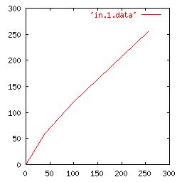
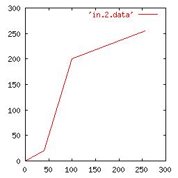
| Contrast Stretching

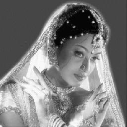
Original Image
|
|
|
Contrast Enhanced Image
|
Excessive Enhacement
|

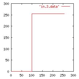
Binary Stated Function (Thresholding)
|
|
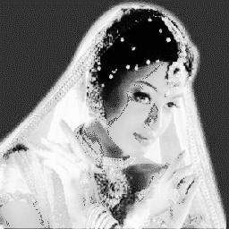
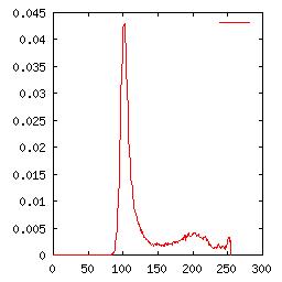
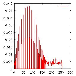
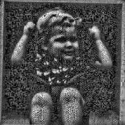
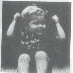
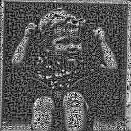
Global Histogram Equalization
|
|

Original Image
|

Equalized Image
|
|
Local Histogram Equalization
For Mask Size 21

|
|

Original Image
|
Equalized Image
|
For Mask Size 9

|
|
Original Image
|
Equalized Image
|
|
|
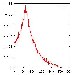
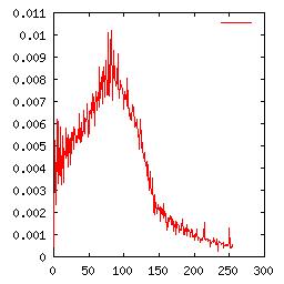
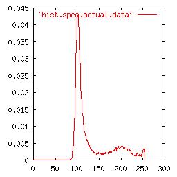
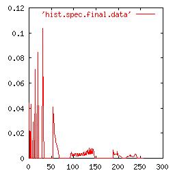
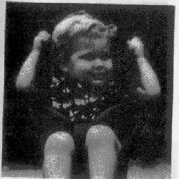
Histogram Specification
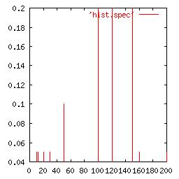
The Input Histogram Specification
|
|

Original Image
|
Equalized Image
|
|
|
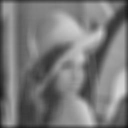
Smoothing Filter (Using Averaging)

The Input Image

For Mask Size 3
|
For Mask Size 9
|
For Mask Size 15
|

The Input Image
For Mask Size 3
|
For Mask Size 5
|

For Mask Size 9
|
|
|
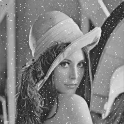
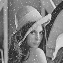
Smoothing Filter (Using Median)

The Input Image
For Mask Size 3
|

For Mask Size 9
|

For Mask Size 13
|

The Input Image

For Mask Size 3
|

For Mask Size 5
|

For Mask Size 9
|
|
|
Highboost Filter

The Input Image
Parameter A=1
|
Parameter A=1.5
|
Parameter A=2
|
Frequency Domain Methods
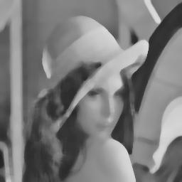
This part of the assignment deals with the frequency domain methods of image enhancement. This
method is computationally much more expensive than the spatial methods. However frequency domain
analysis offers a different perpective of the same problem. In the first part a plot of the number of
points versus time taken for FFT and FFT inverse calculation for a particular image is shown. In the
other parts the effect of an ideal HPF and LPF on an image are seen along with the effect of Butterworth
HPF and LPF. Finally the last part shows the effect of translation and rotation on the FFT of an image.
Translation of an image in the spatial domain only changes the phase of the fourier transform, thus
we donot observer any changes in the magnitude plots shown.
|
FFT and Inverse FFT Time/No. of Point Characterstics

Input Image (size was varied)
|
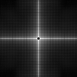
Fourier Transform of Input
|
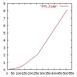
Time(secs)/No. of Points Characterstics
|
|
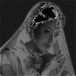
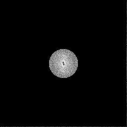
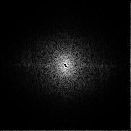
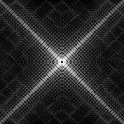
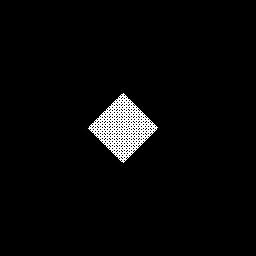
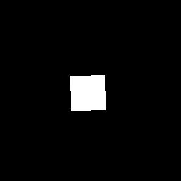
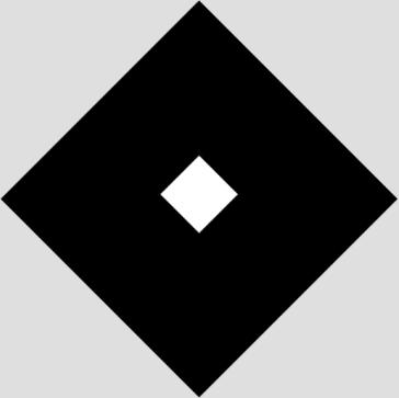
Ideal Low Pass Filter

Input Image for Ideal LPF
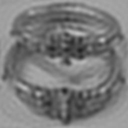
Output Image (Cutoff at 20)
|

Output Image (Cutoff at 30)
|
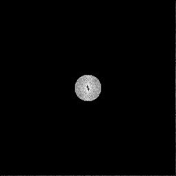
Fourier Transform of Output Image
|
Fourier Transform of Output Image
|
|
|
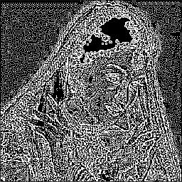
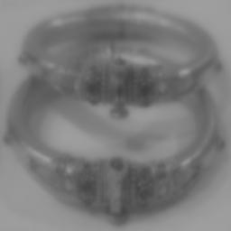
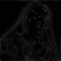
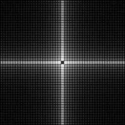
Ideal High Pass Filter
Input Image for Ideal HPF
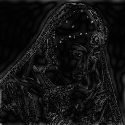
Output Image (Cutoff at 10)
|
Output Image (Cutoff at 30)
|

Fourier Transform of Output Image
|
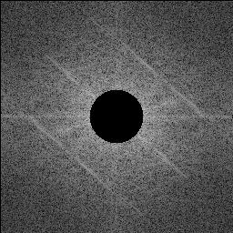
Fourier Transform of Output Image
|
|
|
Butterworth Low Pass Filter
Input Image for Butterworth LPF
Output Image (D0=50, N=2)
|

Output Image (D0=80, N=1)
|
Fourier Transform of Output Image
|
Fourier Transform of Output Image
|
|
|
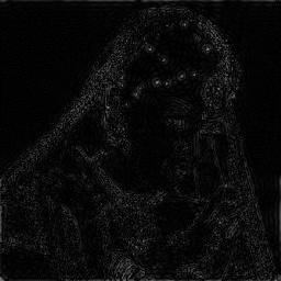
Butterworth High Pass Filter

Input Image for Butterworth HPF
Output Image (D0=3, N=3)
|
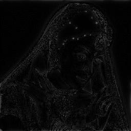
Output Image (D0=10, N=1)
|
Fourier Transform of Output Image
|
Fourier Transform of Output Image
|
|
|
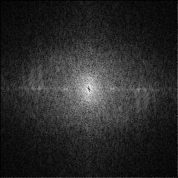
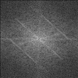
Rotation of Fourier Transform

Original Image
|

Original Image Rotated by 45 degrees
|

Fourier Transform of Original Image
|
Fourier Transform of Rotated Image
|
|
|
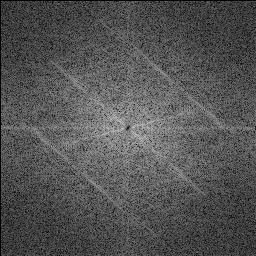
Translation of Fourier Transform
Original Image
|
Original Image Translated by Some Amount
|
Fourier Transform of Original Image
|
Fourier Transform of Translated Image (no change)
|
|
|
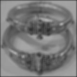
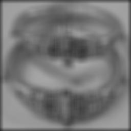
Comparison with ImageMagick Routines
As part of the assignment it was asked to study how the tools developed compares with a
professional quality library both in terms of quality of results obtained and
in performance. This comparative study is elaborated below. From the numbers obtained we can observe
that in most of the cases the tool developed performs better than the ImageMagick routines. However
for a mask size of 9 in median filter, there seems to be some problem with ImageMagick, since the results
obtained also donot show any considerable change (between mask size 3 and 9). For the blur case
the tool developed performs far better than ImageMagick library routines mainly due to the mask movement
optimizations done. A comparison of the results obtained can be made after looking at the images.
|
| Median Filter |
| | Mask Size=3 | Mask Size=9 |
| My Tool | 0.520s | 1.740s |
| ImageMagick | 2.400s | 19.880s |
|
|
| Rotate |
| | Angle=45 | Angle=90 |
| My Tool | 0.440s | 0.390s |
| ImageMagick | 1.030s | 0.180s |
|
|
| Blur |
| | Mask Size=3 | Mask Size=9 | Mask Size=17 |
| My Tool | 0.360s | 0.910s | 1.570s |
| ImageMagick | 0.290s | 1.040s | 4.200s |
|
|
| Equalize |
| | Global |
| My Tool | 0.33s |
| ImageMagick | 0.11s |
|
|
|
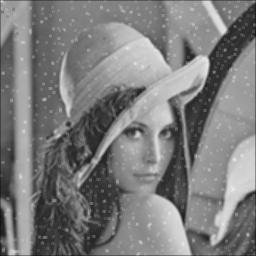
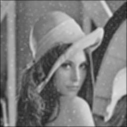
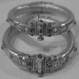
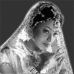
These two input images were used for obtaining the results shown below
Median Filter
|
|
| | Mask Size=3 | Mask Size=9 |
| My Tool |
 |
 |
| ImageMagick |
 |
 |
|
Rotate
|
|
| | Angle=45 | Angle=90 |
| My Tool |
 |
 |
| ImageMagick |
 |
 |
|
Blur
|
|
| | Mask Size=3 | Mask Size=9 | Mask Size=17 |
| My Tool |
 |
 |
 |
| ImageMagick |
 |
 |
 |
|
Equalize
|
|
| | Global |
| My Tool |
 |
| ImageMagick |
 |
|
|
|

